Case Study (IRIS PLANT) :
SKLearrn (K-Nearest Neighbors (K-NN))
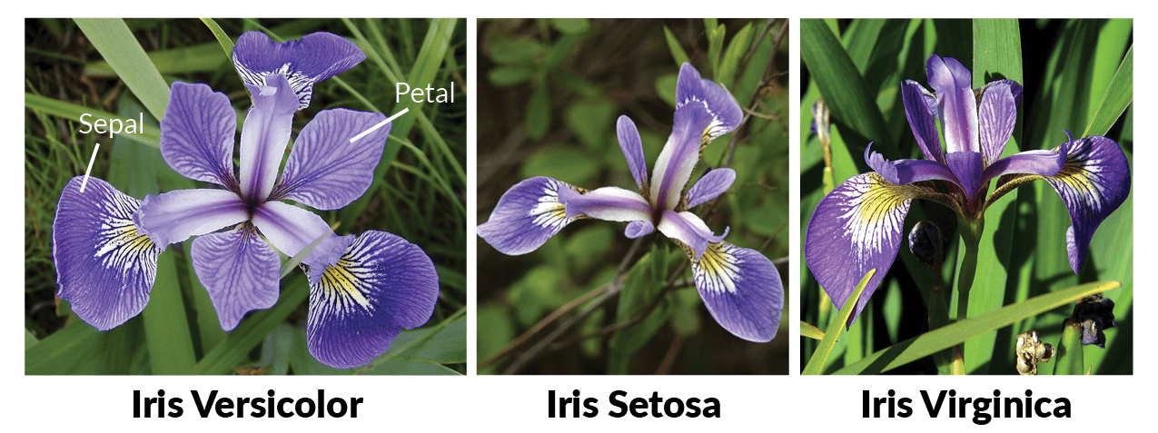
The data set contains 3 classes of 50 instances each, where each class refers to a type of iris plant. The attribute to be predicted is the class of iris plant. The classes are as follows: 1. Iris Setosa, 2. Iris Versicolour, 3. Iris Virginica
There are 4 features:
- sepalLength: sepal length in cm
- sepalWidth: sepal width in cm
- petalLength: petal length in cm
- petalWidth: petal width in cm
There are 3 classes represneting class label of iris flower {1,2,3}
- Iris Setosa
- Iris Versicolour
- Iris Virginica
Dr. Ryan @STEMplicity
Importing the Relevant Libraries
In [1]:
import numpy as np
import pandas as pd
import matplotlib.pyplot as plt
import seaborn as sns
sns.set()
Importing the Dataset
In [2]:
url = "https://datascienceschools.github.io/Machine_Learning/Classification_Models_CaseStudies/Iris.csv"

df = pd.read_csv(url)

df.head()
Out[2]:
Exploring the Dataset
ScatterPlot
In [3]:
plt.figure(figsize=(10,10))

plt.subplot(2,2,1)
sns.scatterplot(df['SepalLengthCm'], df['SepalWidthCm'], hue = df['Species'])

plt.subplot(2,2,2)
sns.scatterplot(df['PetalLengthCm'], df['PetalWidthCm'], hue = df[ 'Species'])

plt.show()

Violinplot
In [4]:
f, ax = plt.subplots(2,2, figsize=(10,10))

f00 = sns.violinplot(df['Species'], df['PetalLengthCm'], ax=ax[0,0])

f01 = sns.violinplot(df['Species'],df['PetalWidthCm'], ax=ax[0,1])

f10 = sns.violinplot(df['Species'], df['SepalLengthCm'], ax=ax[1,0])

f11 = sns.violinplot(df['Species'],df['SepalWidthCm'], ax=ax[1,1])

Pairplot
In [5]:
sns.pairplot(df, hue = 'Species')

plt.show()

Heatmap
In [6]:
corr = df.corr()

matrix = np.triu(corr)

sns.heatmap(corr, annot=True, mask = matrix)

plt.show()

Declaring the Dependent & the Independent Variables
In [7]:
X = df.iloc[:, :-1].values

y = df.iloc[:, -1].values
Label Encoding the Dependent Variable
In [8]:
from sklearn.preprocessing import LabelEncoder

le = LabelEncoder()

y = le.fit_transform(y)
Splitting the Dataset into the Training Set and Test Set
In [9]:
from sklearn.model_selection import train_test_split

X_train, X_test, y_train, y_test = train_test_split(X, y, test_size = 0.20, random_state = 1)
Feature Scaling
from sklearn.preprocessing import StandardScaler
sc = StandardScaler()
X_train = sc.fit_transform(X_train)
X_test = sc.transform(X_test)
Training the K-Nearest Neighbors Model
In [10]:
from sklearn.neighbors import KNeighborsClassifier

model = KNeighborsClassifier(n_neighbors = 5, metric = 'minkowski', p = 2)

model.fit(X_train, y_train)
Out[10]:
Predicting the Test Set Results
In [11]:
y_pred = model.predict(X_test)
Confusion Matrix
In [12]:
from sklearn.metrics import confusion_matrix, accuracy_score

cm = confusion_matrix(y_test, y_pred)

accuracy = accuracy_score(y_test, y_pred)

print("Accuracy is: {:.2f} %".format(accuracy*100))

sns.heatmap(cm, annot=True, fmt="d")

plt.show()

Classification Report
In [13]:
from sklearn.metrics import classification_report

print(classification_report(y_test,y_pred))
k-Fold Cross Validation
In [14]:
from sklearn.model_selection import cross_val_score

accuracies = cross_val_score(estimator = model, X = X_train, y = y_train, cv = 10)

print("Accuracy: {:.2f} %".format(accuracies.mean()*100))

print("Standard Deviation: {:.2f} %".format(accuracies.std()*100))